C++ Class for InfluxDB v1.8

I use InfluxDB v1.8 a lot and using the bash script (to be precise, InfluxDB API using curl in bash shell) to push data is kind of inconvenient, especially for C++ program development.

So, I did some study and develop a C++ Class for it. It is much faster and also easy to use. Here are the link

https://fsunuc.physics.fsu.edu/git/rtang/FSUDAQ/src/branch/master/DAQ/influxdb.h
https://fsunuc.physics.fsu.edu/git/rtang/FSUDAQ/src/branch/master/DAQ/influxdb.cpp

The usage is quite simple,

#include "influxdb.h"

InfluxDB * influx = new InfluxDB("http://localhost:8086")

//if no database, create one
influx->CreateDatabase("database_name");

//Add data point, the data will be saved in the class as a buffer.
for( int i = 0; i < 100 ; i++){
  influx->AddDataPoint("Measurement,tag1=" + std::string(i) + ",tag2=haha value=" + to_string(i*2));
}

//Write data 
influx->WriteData("database_name");

//Clear buffer
influx->ClearDataPointsBuffer();

In a local 1GB network, it writes 64 data points at once as fast as 500 msec.

Web-based HELIOSmatics

There are 2 main tools for the kinematic simulation or calculation for the HELIOS spectrometer. One is using MS Excel, and another one is using CERN ROOT with Monte Carlo events generation.

They work great after downloaded and with MS Excel, not Libre spreadsheet. But a problem is, whenever the code got updated, the user need to update it or download it again. Another disadvantage is on the CERN ROOT simulation, it requires few configuration files. When users need to preform multiple difference reactions and settings, it is not so convivence. In fact, the fundamental layer of the simulation code support different file names, but the GUI does not.

Now I moved the simulation on the web. The calculation mostly done with JavaScript, and plotting by Plotly. The DWBA and Monte Carlo simulation is using CGI python interface to reuse the code developed in C++, like retrieving the mass, calling the DWBA code, etc.

The reason it can be put on the web is the collaboration between FSU and FRIB on the SOLARIS project.

Cheat sheet on C++

Check g++ supports which C++ version

gcc -v --help 2> /dev/null | sed -n '/^ -std=([^<][^ ]+)./ {s//\1/p}'

the above command is from this stack overflow.

Pointer

int haha = 1;
//creation of pointer or "address" : Type/Class * XXX
//should view as (Type/Class *) XXX
int * address_of_haha = &haha; //address of a non-pointer (&) 
int kaka = *address_of_haha; //context of an address (*)
//pointer of an array
int jaja[5] = {1, 2, 3, 4, 5};
int * papa = jaja; //papa is the address of jaja[0]
// *papa = papa[0] = jaja[0]
// *(papa+1) = papa[1] = jaja[1]

Clone a pointer

a single object

Class * haha = new Class();
Class * kaka = new Class(*haha);

or

Class * haha = new Class();
Class * kaka = new Class();
*kaka = *haha; // only copy the haha[0], if haha is an array.

to clone a pointer array

Class * haha = new Class();
Class * kaka = NULL;
std::memcpy(kaka, haha, sizeof(haha));

cxxx vs xxx.h

• cxxx are c++ library using namespace
• xxx.h are c library using global variable
• <cmath> defines the relevant symbols under the std namespace; <math.h> defines them globally.

Stack vs Heap

in a very rough sense, stack memory is

• static memory that memory allocation happened when the contained function is called.
• the size of the memory is known to the compiler.
• the function is over, the memory is de-allocated.
• memory allocation and de-allocation is faster, compare to heap memory.

these are stack memory:

int haha;
int kaka[5];

in a very rough sense, heap memory is opposite to stack. So,

• dynamic memory, memory allocation happened when the “new” operator is called.
• the size of the memory is not know to the compiler.
• need manually to de-allocated.

To allocate a heap memory:

int * haha = new int[5];

Delete a pointer

whenever a pointer array is created using [], use delete []

int * haha = new int [10];
delete [] haha;

int ** kaka = new int *[10];
for(int i = 0; i < 10; i++ ) kaka[i] = new int;
for(int i = 0; i < 10; i++ ) delete kaka[i];
delete [] kaka;
 

new vs malloc

malloc() does not call the constructor. malloc() use free() to de-allocate memory. new use delete to free memory.

int * haha = (int *) malloc (sizeof(int) * 5);
free(haha); // or delete haha;
int * kaka = new int[5];
delete [] kaka;

Simple agglomerative single-linkage clustering

The problem is that, there are serval parallel curves and we have to fit the curves. Or, for a set of family of cruve

where is the function we want to fit, is the error, is the offset for each line. This is something like this:

---

The function I am dealing with is something is a quadratic plus some high order fluctuation, .

I tried many ways to “convert” the problem in to ordinary fitting. One way is using the least-square method with a threshold and maximize number of points fitted. The idea is, pick a point and compare the distance from all lines with initial guessing parameters, if the minimum distance is smaller than the threshold, it counted. By maximizing the number of points counted and minimized the total square distance via searching thought the whole parameter space, we can least-squared fit the data. However, searching the whole parameter space could be time consuming. And so far, I did not know any good way to solve this “finding minimum of an complicated function” .

---

Another way is clustering, since each curve is an obvious cluster in human eyes. However, how to let the computer know is the problem. I tried neural network, but I failed to do the unsupervised learning. Thus, I turn to a more conventional method — Agglomerative single-linkage clustering. This method is well demonstrated in the wiki. A dendrogram is the final product of the algorithm. From the dendrogram, we can cluster the data into many clusters.

I know that the scipy package for python has the fast algorithm, but I prefer C++, and cannot find a simple code. So, I wrote my code and show the result in here.

---

First, we need a distance metric, a definition of distance. I choose the Euclidean distance, which is

Once we calculated the distance matrix that each element is

Then, the smallest distance pair is found, say, . Then, we need to calculated the new distance matrix that show the new distance for the cluster to the rest of the points, and how this is done depends on single-linkage, complete-linkage, or average-linkage.

In the matrix sense, the new distance matrix will be 1-row and 1 column smaller. But in the implementation, for simplicity, keep the matrix size to be the same and simply fill the row and column with larger index with nan. in this way, the index or the id of each point with not change, and the cluster id will be the smaller id of the points in the cluster.

For example, ten points

The distance matrix is

I set the distance function be . The closed pair is (4,5), and the distance is 0.090961. And “4” will be the cluster id.

The new distance matrix is

We set row and column 5 to be nan. the new column and row 4 will be using single-linkage. The single-linkage is taking the minimum distances to the cluster. For complete-linkage, the distance to the cluster is the maximum distances. In the below example, the (a,b) formed a pair. The distance of the point c to pair (a,b) could be the minimum, the maximum, or the average of (a,c) and (b,c).

Back to the example, lets take (0,4) and (0, 5). This new distance will be the minimum among the two. min(0.6238, 0.5939) = 0.5939. Same procedure apply for the others.

After 9 iterations, all matrix elements becomes nan and the clustering complete. The sequence of the pair is

The corresponding dendrogram is

From the dendrogram, it is easily to divide the data points into 2 clusters.

---

The C++ code for CERN root is:

double distant(double x1, double y1, double x2, double y2 ){
  return sqrt( (x1-x2)*(x1-x2) + (y1-y2)*(y1-y2)) ;
}

struct MinPos{
  double min;
  vector<int> pos;
};

MinPos FindMin(double *D, int size){

  MinPos mp;

  mp.min = 1e9;
  for( int i = 0 ; i < size; i++){
    for( int j = i ; j < size; j++){
      if( D[i*size+j] < mp.min ) {
        mp.min = D[i*size+j];
        mp.pos = {i, j};
      }
    }
  }

  if( mp.min == 1e9 ) mp.min = TMath::QuietNaN();

  return mp;
}

double * ReduceDMatrix(double *D, int size, MinPos mp){

  double * Dnew = new double [size*size];
  for( int i = 0 ; i < size; i++){
    for( int j = 0 ; j < size; j++){
      if( i == mp.pos[0] || i == mp.pos[1]) {
        Dnew[i*size+j]= TMath::Min( D[mp.pos[0]*size+j] , D[mp.pos[1]*size+j] );
      }else if( j == mp.pos[0] || j == mp.pos[1]){
        Dnew[i*size+j]= TMath::Min( D[i*size+mp.pos[0]] , D[i*size+mp.pos[1]] );
      }else{
        Dnew[i*size+j] = D[i*size+j];
      }
    }
  }
  for( int i = 0 ; i < 2 ; i++){  
    for( int j = 0 ; j < 2 ; j++){
      Dnew[mp.pos[i]*size+mp.pos[j]] = TMath::QuietNaN();
    }
  }
  for( int j = 0; j < size; j++) Dnew[mp.pos[1] * size + j ] = TMath::QuietNaN();
  for( int i = 0; i < size; i++) Dnew[i * size + mp.pos[1] ] = TMath::QuietNaN();

  return Dnew;

}

int main(){

  ///============== Generate data
  const int n = 10;
  double x[n], y[n], ey[n], oy[n];

  for( int i = 0; i < n; i++){
    x [i] = gRandom->Rndm();
    ey[i] = gRandom->Gaus(0,0.1);
    oy[i] = gRandom->Integer(2);
    y [i] = x[i] + ey[i] + 5* oy[i];    
  }

  ///================ Clustering (agglomerative, single-linkage clustering 
  double * D1 = new double [n*n];
  for( int i = 0 ; i < n; i++){
    for( int j = 0 ; j < n; j++){
      if( i ==j ) {
        D1[i*n+j] = TMath::QuietNaN();
        continue;
      }
      D1[i*n+j] = distant(x[i], y[i], x[j], y[j]);
    }
  }

vector<vector<int>> dendrogram;
  vector<double> branchLength;

  MinPos mp = FindMin(D1, n);
  dendrogram.push_back(mp.pos);
  branchLength.push_back(mp.min/2.);

  double * D2 = D1;
  int count = 2;
  do{
    D2 = ReduceDMatrix(D2, n, mp);
    mp = FindMin(D2, n);
    if( TMath::IsNaN(mp.min) ){
      break;
    }else{
      dendrogram.push_back(mp.pos);
      branchLength.push_back(mp.min/2.);
    }
    count ++;
  }while( !TMath::IsNaN(mp.min) );

  ///================= find the group 1 from the dendrogram.
  int nTree = (int) dendrogram.size() ;
  vector<int> group1;
  for( int i = nTree -1 ; i >= 0 ; i--){
    if( i == nTree-1 ){
      group1.push_back(dendrogram[i][0]);
    }else{
      int nG = (int) group1.size();
      for( int p = 0; p < nG; p++){
        if( group1[p] == dendrogram[i][0] ) {
              group1.push_back(dendrogram[i][1]);
        }
      }
    }
  }

}

Using this code, for two parallel lines,

another data set:

Momentum distribution From Woods-Saxon potential

In this post, we derived the transformation between radial distribution and momentum distribution. This is a simple “Fourier Transform” in 3D with spherical Bessel function. In that post we also plot some simple functions.

The effective potential for most nuclei can be approximated (or well described) using the Woods-Saxon potential. Here we study the 15C, find the radial wave functions and the corresponding momentum distributions.

There are many way to calculate the radial function for a give set of Woods-Saxon parameters, using C++ code, MS excel, or Mathematica. In this post, I will use Mathematica. I found that MS Excel has the Bessel function, but it only accept integer n, but spherical Bessel needs half integer n, so it is not easy for calculating the momentum distribution.

In Mathematica, solving the Schrodinger equation for the radial part is extremely easy, for give energy , angular momentum , total spin

sol = NDSolve[{u''[
r] == (2 m)/hbar^2 (V0/(1 + Exp[(r - R0)/a0]) - 
1/r (Exp[(r - RSO)/aSO] VSO)/(a0 (1 + Exp[(r - RSO)/aSO)]^2)
LS - T) u[r] + (L (L + 1))/r^2 u[r], u[0] == 0, u'[0] == 1}, 
u, { r, 0, 30}];

where is the potential depth in MeV, is the hald-radius in fm, is the diffusiveness parameter in fm, and the subscript for central and spin-orbit. is the LS coupling factor. is the reduced radial function.

The normalization of the reduced radial function is

---

Usually, we don’t know the energy for a give state, we have to scan through all possible energy from . When the energy is not the eigen energy, the tail of the wave function will diverge and oscillate with respect to the energy. Thus, we can use this property to find the eigen energy that the tail of the wave function is flat.

In here, I am requiring the sum to be minimum.

For 15C, the single particle energies for the 1s1/2 and 0d5/2 is known from the 14C(d,p) reaction, which are -1.2181 MeV and -0.4741 MeV, respectively.

After searching for best fit parameters, I found

are best fit. The energies of different states are:

Orbital	Energy (WS) [MeV]	Energy (exp) [MeV]
0s1/2	-25.634
0p3/2	-12.522
0p1/2	-10.351
1s1/2	-1.210	-1.2181
0d5/2	-0.463	-0.474

And, I have the radial function.

We can see that, the 1s1/2 orbital has largest radial distribution and the 0s1/2 has the smallest.

Next, we transform the radial distribution to the momentum distribution. The unit conversion is that

In the above figure, we scaled the distribution so that they have similar magnitude. We can see, the momentum distribution is smallest for the 1s1/2 as expected.

It is interesting that the momentum spread of the 0s1/2 and 1s1/2 are very different, the spread of the 0s1/2 is almost 3 times more than that of the 1s1/2, and that of the p-wave also about double.

And the d-wave momentum distribution has 2 bumps, this looks something wrong. (??? I am no solid answer for that. I suspect this is related to the tail of the wave function, when the tail is not zero, the spherical Bessel J times r^2 will magnify the tail. )

---

The radial solution of the Woods-Saxon potential (or the Schrodinger equation?) for the bound state is always take this form:

where is the short range behaviour, is the long range behaviour, and is a modifier for the middle part of the function.

Lets assume the for simplicity.

The momentum distribution using this simplified radial function is

Normalized with

Here are the plot with for

the is similar to orbital.

The momentum distribution is good for distinguish and , but not so good for higher .

And it is counter intuitive that more spread of the radial function, the momentum distribution also spread out more. I guess the effect of the angular momentum has to take into account. For same , more spread of momentum still means the radial spread is smaller.

Memo on doing Shell model calculation with OXBASH

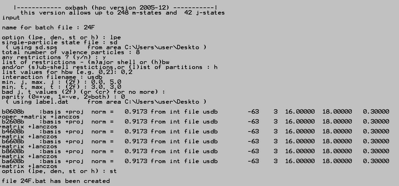
I am using the window version of the code, version 2005-12.

---

To calculate the configuration, for example 24F. In the command line type

>shell

It will then guide you though

right after the file name, in the option, for “lpe”, you can also add “lpe, 1” for only 1 state. The default is calculate the first 10 energy state for each spin-isospin.

After running the 24F.bat, you will have a lot of file generated. The most important files are the lpe file. It contains the calculation result. According to the help manual, the file name is like:

---

To calculate the spectroscopic factor, i.e. the overlap of two wave functions.

Suppose I want to calculate the spectroscopic factor for the 23F(d,p)24F reaction.

The recipe is follow:

1. Calculate the ground state of 23F using the “lpe, 1”, and mark down the file name like : b5507b
2. Calculate the states of 24F and make down any file name, e.g. : b0608b
3. using the open “den”, and “1”, the core wave function should be the 23F, and the overlap wave function should be the 24F.

The most important output file are the lsf files.

---

I wrote two simple c++ code for extracting the excited states and the spectroscopic factors form the above “method”.

https://github.com/goluckyryan/programmings/tree/master/cpp/oxbash

3j, 6j, 9j-symbol for C++

Since I cannot find a odd c++ code ( < c++11 ) for the calculation of those j-symbol, I made one for myself!

The code just using the formula which you can find in wiki or here. So, the code is not optimized, but for simple calculation, I guess it does not matter. Also, I checked, in my pc, calculate 1000 9-j symbols only take 1 or 2 sec.

The program first build

1. factorial
2. Clebsch–Gordan coefficient
3. 3-j symbol
4. 6-j symbol
5. 9-j symbol

#include <stdlib.h>
#include <cmath>
#include <algorithm>

using namespace std;

double factorial(double n){
  if( n < 0 ) return -100.;
  return (n == 1. || n == 0.) ? 1. : factorial(n-1) * n ;
}

double CGcoeff(double J, double m, double J1, double m1, double J2, double m2){
  // (J1,m1) + (J2, m2) = (J, m)

  if( m != m1 + m2 ) return 0;

  double Jmin = abs(J1 - J2);
  double Jmax = J1+J2;

  if( J < Jmin || Jmax < J ) return 0;

  double s0 = (2*J+1.) * factorial(J+J1-J2) * factorial(J-J1+J2) * factorial(J1+J2-J) / factorial(J+J1+J2 + 1.);
  s0 = sqrt(s0);

  double s = factorial(J +m ) * factorial(J -m);
  double s1 = factorial(J1+m1) * factorial(J1-m1);
  double s2 = factorial(J2+m2) * factorial(J2-m2);
  s = sqrt(s * s1 * s2);

  //printf(" s0, s = %f , %f \n", s0, s);

  int kMax = min( min( J1+J2-J, J1 - m1), J2 + m2);

  double CG = 0.;
  for( int k = 0; k <= kMax; k++){
    double k1 = factorial(J1+J2-J-k);
    double k2 = factorial(J1-m1-k);
    double k3 = factorial(J2+m2-k);
    double k4 = factorial(J - J2 + m1 +k);
    double k5 = factorial(J - J1 - m2 +k);
    double temp = pow(-1, k) / (factorial(k) * k1 * k2 * k3 * k4 * k5);
    if( k1 == -100. || k2 == -100. || k3 == -100. || k4 == -100. || k5 == -100. ) temp = 0.;

    //printf(" %d | %f \n", k, temp);
    CG += temp;
  }

  return s0*s*CG;

}

double ThreeJSymbol(double J1, double m1, double J2, double m2, double J3, double m3){

  // ( J1 J2 J3 ) = (-1)^(J1-J2 - m3)/ sqrt(2*J3+1) * CGcoeff(J3, -m3, J1, m1, J2, m2) 
  // ( m1 m2 m3 )

  return pow(-1, J1 - J2 - m3)/sqrt(2*J3+1) * CGcoeff(J3, -m3, J1, m1, J2, m2);

}

double SixJSymbol(double J1, double J2, double J3, double J4, double J5, double J6){

  // coupling of j1, j2, j3 to J-J1
  // J1 = j1
  // J2 = j2
  // J3 = j12 = j1 + j2
  // J4 = j3
  // J5 = J = j1 + j2 + j3
  // J6 = j23 = j2 + j3

  //check triangle condition
  if( J3 < abs(J1 - J2 ) || J1 + J2 < J3 ) return 0; 
  if( J6 < abs(J2 - J4 ) || J2 + J4 < J6 ) return 0;
  if( J5 < abs(J1 - J6 ) || J1 + J6 < J5 ) return 0;
  if( J5 < abs(J3 - J4 ) || J3 + J4 < J5 ) return 0;

  double sixJ = 0;

  for( float m1 = -J1; m1 <= J1 ; m1 = m1 + 1){
    for( float m2 = -J2; m2 <= J2 ; m2 = m2 + 1){
      for( float m3 = -J3; m3 <= J3 ; m3 = m3 + 1){
        for( float m4 = -J4; m4 <= J4 ; m4 = m4 + 1){
          for( float m5 = -J5; m5 <= J5 ; m5 = m5 + 1){
            for( float m6 = -J6; m6 <= J6 ; m6 = m6 + 1){

              double f = (J1 - m1) + (J2 - m2) + (J3 - m3) + (J4 - m4) + (J5 - m5) + (J6 - m6);

              double a1 = ThreeJSymbol( J1, -m1, J2, -m2, J3, -m3); // J3 = j12 
              double a2 = ThreeJSymbol( J1, m1, J5, -m5, J6, m6); // J5 = j1 + (J6 = j23)
              double a3 = ThreeJSymbol( J4, m4, J2, m2, J6, -m6); // J6 = j23
              double a4 = ThreeJSymbol( J4, -m4, J5, m5, J3, m3); // J5 = j3 + j12

              double a = a1 * a2 * a3 * a4;
              //if( a != 0 ) printf("%4.1f %4.1f %4.1f %4.1f %4.1f %4.1f | %f \n", m1, m2, m3, m4, m5, m6, a);

              sixJ += pow(-1, f) * a1 * a2 * a3 * a4;

            }
          }
        }
      }
    }
  }

  return sixJ;
}

double NineJSymbol( double J1, double J2, double J3, double J4, double J5, double J6, double J7, double J8, double J9){

  double gMin = min( min (min( abs(J1 - J2 ), abs(J4 - J5)) , abs( J4 - J6 )) , abs(J7 - J8));
  double gMax = max( max (max( J1+J2, J4+J5), J3+J6), J7+J8);

  //printf(" gMin, gMax = %f %f \n", gMin, gMax);

  double nineJ = 0;
  for( float g = gMin; g <= gMax ; g = g + 1){
    double f = pow(-1, 2*g) * (2*g+1);
    double s1 = SixJSymbol(J1, J4, J7, J8, J9, g);
    if( s1 == 0 ) continue;
    double s2 = SixJSymbol(J2, J5, J8, J4, g, J6);
    if( s2 == 0 ) continue;
    double s3 = SixJSymbol(J3, J6, J9, g, J1, J2);
    if( s3 == 0 ) continue;
    nineJ += f* s1*s2*s3;
  }

  return nineJ;
}

a GEANT4 Simulation

The GEANT4 program structure was borrow from the example B5. I found that the most confusing part is the Action. Before that, let me start with the main().

GEANT4 is a set of library and toolkit, so, to use it, basically, you add a alot GEANT4 header files on your c++ programs. And, every c++ program started with main(). I write the tree diagram for my simplified exampleB5,

main()
 +- DetectorConstruction.hh
    +- Construct()
       +- HodoscopeSD.hh     // SD = sensitive detector
          +- HodoscopeHit.hh //information for a hit
          +- ProcessHits()   //save the hit information
       +- ConstructSDandField() //define which solid is SD
       +- ConstructMaterials()  //define material
+- PhysicsList.hh  // use FTFP_BERT, a default physics for high energy physics
+- ActionInitialization.hh
   +- PrimaryGeneratorAction.hh // define the particle gun
   +- RunAction.hh // define what to do when a Run start, like define root tree
   +- Analysis.h  // call for g4root.h
   +- EventAction.hh //fill the tree and show some information during an event

 

A GEANT4 program contains 3 parts: Detector Construction, Physics, and Action. The detector construction is very straight forward. GEANT4 manual is very good place to start. The physics is a kind of mystery for me. The Action part can be complicated, because there could be many things to do, like getting the 2ndary beam, the particle type, the reaction channel, energy deposit, etc…

Anyway, I managed to do a simple scattering simulation, 6Li(2mm) + 22Ne(60A MeV) scattering in vacuum. A 100 events were drawn. The detector is a 2 layers plastic hodoscope, 1 mm for dE detector, 5 mm for E detector. I generated 1 million events. The default color code is Blue for positive charge, Green for neutral, Red for negative charge. So, the green rays could be gamma or neutron. The red rays could be positron, because it passed through the dE detector.

The histogram for the dE-TOF is

We can see a tiny spot on (3.15,140), this is the elastics scattered beam, which is 20Ne. We can see 11 loci, started from Na on the top, to H at the very bottom.

The histogram of dE-E

For Mass identification, I follow the paper T. Shimoda et al., Nucl. Instrum. Methods 165, 261 (1979).

I counted the 20Na from 0.1 billion beam, the cross section is 2.15 barn.

 

Command line argument

here i copy form this web page:

http://www.learncpp.com/cpp-tutorial/713-command-line-arguments/

#include <iostream>

int main(int argc, char *argv[])
{
    using namespace std;

    cout << "There are " << argc << " arguments:" << endl;

    // Loop through each argument and print its number and value
    for (int nArg=0; nArg < argc; nArg++)
        cout << nArg << " " << argv[nArg] << endl;

    return 0;
}

where argc store the number of the arguments. it is at least 1, coz it contains the file name. when you type the argument, it will store in argv. in my case, i have a program for Fourier Transform called FFTW.mac

./FFTW.mac ise.dat 1000 abc

thus, ise.dat is the 1st argument, stored in argv[1], 1000 is 2nd, stored in argv[2], abc is 3rd, stored in argv[3]…etc.

simple FFTW C++ code for Complex Fourier Transform

// an input complex array and output complex array

fftw_complex *input, *out;

// define the size of the array 5000 X 2 *)

out = (fftw_complex*) fftw_malloc(5000*2*sizeof(fftw_complex));

input = (fftw_complex*) fftw_malloc(5000*2*sizeof(fftw_complex));

// feed data into the input array 

for(int i=0;i<5000;i++)

{

input[i][0]=dcos[i] ; // dcos[i] is an array that stored raw data of cosine part

input[i][1]=dsin[i] ; // dsin[i] is an array stored raw data of sine part

}

//declare a plan

fftw_plan p;

//define the plan, i don’t know what it is, just copy the code from FFTW manual

p= fftw_plan_dft_1d(5000,input,out,FFTW_FORWARD,FFTW_ESTIMATE);

// execute the plan, or tranform

fftw_execute(p);

// save the data into array Fdata

for(int i=0;i<5000;i++)

{

Fdata[i][0]=out[i][0];

Fdata[i][1]=out[i][1];

}

fftw_destroy_plan(p);

delete [] input;

delete [] out;

//Fourier Transform