spherical harmonic | Nuclear Physics 101

Coulomb Energy for two protons system

March 5, 2020

GoLuckyRyan Basic Coulomb, Coulomb Energy, spherical Bessel, spherical harmonic Leave a comment

From this post and this post, we already have the framework to calculate the energy. The 1-body intersection is zero, as we do not interested on the kinematics energy. And also, suppose we already have the solution for the wave function for a fixed mean-field. Although it is unrealistic, it is a good starting point.

In fact, we have to solve the Schrödinger equation (using Hartree-Fock or numerical solution) with a realistic NN-interaction with and without Coulomb potential, and subtract the difference to get the Coulomb energy.

We have to evaluate the integral

$\displaystyle W = \left<12||12\right> - \left<12||21\right>$

When the 2 protons are in same orbital, the total wavefunction is

$\displaystyle \Psi(1,2) = \frac{1}{\sqrt{2}}\left(\uparrow \downarrow - \downarrow \uparrow \right) \phi(r_1) \phi(r_2)$

The exchange term is zero as the Coulomb operator does not act on the spin part.

$\displaystyle \left<12||12\right> = \sum_{L}^{\infty} \sum_{M=-L}^{L} \frac{4\pi}{2L+1}\int_{0}^{\infty} \int_{0}^{\infty} \phi^2(x) \phi^2(y) \frac{r_<^L}{r_>^{L+1}} x^2 y^2 dx dy \\ \int Y_{lm}^*(1) Y_{LM}^*(1) Y_{lm}(1) d\Omega_1 \int Y_{lm}^*(2) Y_{LM}(2) Y_{lm}(2) d\Omega_2$

For the angular part, from this post or this post, we have

$\displaystyle \int Y_{l_1m_1}^* Y_{LM}^* Y_{l_2m_2} d\Omega = \sqrt{\frac{(2L+1)(2l_1+1)}{4\pi(2l_2+1)}} C_{L0l_10}^{l_20} C_{LMl_1m_1}^{l_2m_2}$

For $l_1 = l_2$ , the Clebsh-Gordon coefficient dictated that $2l \geq L$ , $L = even$ , $M = 0$ .

We use the potential is 3D spherical infinite well with radius $a = 2.2$ fm. the wave function is spherical Bessel function ,

$\phi_n(r ) = \begin{matrix} A j_n(k r) & r < a \\ 0 & r > a \end{matrix}, j_n(ka) = 0$ ,

where $A$ is the normalization factor.

Screenshot 2020-03-05 at 17.48.19.png

The first non-zero root of spherical Bessel Function take the form,

$r_0(n) = 2.96519 + 0.701921\sqrt{n} + 0.993301 n, n < 500$

The energy for the $n$ -th s-state is

$\displaystyle E_n = \frac{\hbar k^2}{2 m_p^2}, k a = r_0(n)$

In Mathematica, the radial calculation can be done as

a=2.2;
R[r_]:=Piecewise[{{SphericalBesselJ[n, r0[n] r], 0 < r < a}, {0, r > 0}}];
A=(NIntegrate[(R[r])^2 r^2, {r, 0, ∞}]])^(-½);
w = NIntegrate[(R[x]R[y])^2 y^L/x^(L+1) x^2 y^2 , {x, 0, ∞}, {y,0, x}] + NIntegrate[(R[x]R[y])^2 x^L/y^(L+1) x^2 y^2 , {x, 0, ∞}, {y,x, ∞}]
W=1.44 A^4 w

The result for first n s-orbital is

Screenshot 2020-03-05 at 17.59.37.png

I also extract the radius for uniformly charged sphere. The trend is reasonable as higher principle number, the wave function is close to the boundary $a = 2.2 \textrm{fm}$ .

Next time, we will work on Woods-Saxon potential.

Evaluation of mutual interaction

October 26, 2017

GoLuckyRyan Math 3-j Symbol, spherical harmonic Leave a comment

We are going to evaluation the integral

$\displaystyle G_{ij}^{hk} = \langle b_i(x) b_h(y) | \frac{1}{r_{xy}} | b_j(x) b_k(y) \rangle$

Recalling the multi-pole expansion,

$\displaystyle \frac{1}{r_{12}} = \sum_{l=0}^{\infty} \frac{4 \pi}{2l+1} \frac{r_{<}^l}{r_{>}^{l+1}} \sum_{m=-l}^{l} Y_{lm}^{*}(\Omega_1) Y_{lm}(\Omega_2)$

and the basis

$b_{nlm}(\vec{r}) = R_{nl}(r) Y_{lm}(\Omega)$

Set an averaged basis

$\displaystyle b_{nl}(\vec{r}) = R_{nl}(r) \frac{1}{\sqrt{2l+1}} \sum_{m=-1}^{l}Y_{lm}(\Omega)$

$\displaystyle \Gamma_{ij}^{hk}(l) = \frac{4 \pi}{2l+1} \sum_{m=-l}^{l} \frac{1}{\sqrt{(2l_i+1)(2l_j+1)(2l_h+1)(2l_k+1)}} \\ \sum_{m_i,m_j}\int Y_{l_i m_i}^{*}(\Omega_1) Y_{l m}^{*}(\Omega_1) Y_{l_j m_j}(\Omega_1) d \Omega_1 \\ \sum_{m_h,m_k} \int Y_{l_h m_k}^{*}(\Omega_2) Y_{l m}(\Omega_2) Y_{l_k m_k}(\Omega_2) d \Omega_2$

In the angular integrals, using Wigner 3-j symbol and the integral

$\displaystyle\int Y_{l_1 m_1}(\Omega) Y_{l m}(\Omega) Y_{l_2 m_2}(\Omega) d \Omega \\= \frac{\sqrt{(2l_1+1)(2l+1)(2l_2+1)}}{\sqrt{4\pi}} \begin{pmatrix} l_1 & l & l_2 \\ 0 & 0 & 0 \end{pmatrix} \begin{pmatrix} l_1 & l & l_2 \\ m_1 & m & m_2 \end{pmatrix}$

$Y_{lm}^{*}(\Omega) = (-1)^m Y_{l(-m)}(\Omega)$

$\displaystyle \begin{pmatrix} l_1 & l & l_2 \\ m_1 & m & m_2 \end{pmatrix} = (-1)^{l_1+l+l_2} \begin{pmatrix} l_1 & l & l_2 \\ -m_1 & -m & -m_2 \end{pmatrix} \\ =(-1)^{l_1+l+l_2} \begin{pmatrix} l_1 & l_2 & l \\ m_1 & m_2 & m \end{pmatrix}$

we have

$\displaystyle\int Y_{l_i m_i}^{*}(\Omega) Y_{l m}^{*}(\Omega) Y_{l_j m_j}(\Omega) d \Omega \\= (-1)^{m_j} \frac{\sqrt{(2l_i+1)(2l+1)(2l_j+1)}}{\sqrt{4\pi}} \begin{pmatrix} l_i & l & l_j \\ 0 & 0 & 0 \end{pmatrix} \begin{pmatrix} l_i & l & l_j \\ m_i & m & -m_j \end{pmatrix}$

$\displaystyle\int Y_{l_h m_h}^{*}(\Omega) Y_{l m}(\Omega) Y_{l_k m_k}(\Omega) d \Omega \\= (-1)^{m_h} \frac{\sqrt{(2l_h+1)(2l+1)(2l_k+1)}}{\sqrt{4\pi}} \begin{pmatrix} l_h & l & l_k \\ 0 & 0 & 0 \end{pmatrix} \begin{pmatrix} l_h & l & l_k \\ -m_h & m & m_k \end{pmatrix}$

Thus,

$\displaystyle \Gamma_{ij}^{hk}(l) = \sum_{m=-l}^{l} \sum_{m_i,m_j } (-1)^{m_j} \begin{pmatrix} l_i & l_j & l \\ 0 & 0 & 0 \end{pmatrix} \begin{pmatrix} l_i & l_j & l \\ m_i & -m_j & m \end{pmatrix} \\ \sum_{m_h,m_k} (-1)^{m_h} \begin{pmatrix} l_h & l_k & l \\ 0 & 0 & 0 \end{pmatrix} \begin{pmatrix} l_h & l_k & l \\ -m_h & m_k & m \end{pmatrix}$

The 3-j symbol restricted that

$l_i+l_j+l = even$

$l_h+l_k+l = even$

$m_i-m_j + m = 0, |m_i| \leq l_i , |m_j| \leq l_j$

$-m_h + m_k +m = 0, |m_h| \leq l_h , |m_k| \leq l_k$

I guess it is the most simplified formula for the angular part.

The total integral is

$\displaystyle G_{ij}^{hk} = \sum_{l=0}^\infty \Gamma_{ij}^{hk}(l) \langle R_i(x) R_h(y) | \frac{r_<^l}{r_>^{l+1}} |R_j(x) R_k(y) \rangle$

The angular integral imposes condition for $l$ .

I am not sure this is a correct way to treat the problem.

First, the averaged basis is still an energy eigen state. It is not the eigen state for the angular part. So, this averaging could introduces an error and we should reminded that this is an approximation. But in the perturbation view point, this averaged basis is still valid.

Second thing is, the sum

$\displaystyle P_{(l_i m_i) (l_j m_j)}^{(l_h m_h)(l_k m_k)}(l) = \sum_{m=-l}^{l} \langle Y_{l_i m_i}|Y_{lm}^*|Y_{l_j m_j}\rangle \langle Y_{l_h m_h}|Y_{lm}|Y_{l_k m_k}\rangle$

is not symmetry for exchange of $i, j, h,k$ in general. For example,

$\displaystyle \frac{-1}{3}=P_{(1-1) (00)}^{(11)(00)}(1) {\neq} P_{(00)(1-1)}^{(11)(00)}(1) = 0$

This is a very uprising result that the mutual interaction dependent on the magnetic quantum number. Thus, in detail, we should use $n l m m_s$ as a basis.

Third, the sum $P_{ij}^{hk}(l)$ is depend on $l$ . The mutual interaction require us to sum all possible $l$ .

Fourth, the coupling between 1s2p triplet state, the total spin is $S = 1$ , total L is $L = 1$ , and the total angular momentum can be $J = 0, 1, 2$ . In our treatment, we did not coupled the angular momentum in the calculation explicitly. In fact, in the integral of the spherical harmonic, the coordinate are integrated separately, and the coupling seem to be calculated implicitly. I am not sure how to couple two spherical harmonics with two coordinates.

Review on rotation

August 15, 2017

GoLuckyRyan Basic, review angular momentum, Clebsch-Gordon, Eigen System, Euler, Fourier transform, Laplacian, rotation, spherical harmonic, Wigner-D Leave a comment

The rotation of a vector in a vector space can be done by either rotating the basis vector or the coordinate of the vector. Here, we always use fixed basis for rotation.

For a rigid body, its rotation can be accomplished using Euler rotation, or rotation around an axis.

Whenever a transform preserves the norm of the vector, it is a unitary transform. Rotation preserves the norm and it is a unitary transform, can it can be represented by a unitary matrix. As a unitary matrix, the eigen states are an convenient basis for the vector space.

We will start from 2-D space. Within the 2-D space, we discuss about rotation started by vector and then function. The vector function does not explicitly discussed, but it was touched when discussing on functions. In the course, the eigen state is a key concept, as it is a convenient basis. We skipped the discussion for 3-D space, the connection between 2-D and 3-D space was already discussed in previous post. At the end, we take about direct product space.

In 2-D space. A 2-D vector is rotated by a transform R, and the representation matrix of R has eigen value

$\exp(\pm i \omega)$

and eigenvector

$\displaystyle \hat{e}_\pm = \mp \frac{ \hat{e}_x \pm i \hat{e}_y}{\sqrt{2}}$

If all vector expand as a linear combination of the eigen vector, then the rotation can be done by simply multiplying the eigen value.

Now, for a 2-D function, the rotation is done by changing of coordinate. However, The functional space is also a vector space, such that

$a* f_1 + b* f_2$ still in the space,
exist of unit and inverse of addition,
the norm can be defined on a suitable domain by $\int |f(x,y)|^2 dxdy$

For example, the two functions $\phi_1(x,y) = x, \phi_2(x,y) = y$ , the rotation can be done by a rotational matrix,

$\displaystyle R = \begin{pmatrix} \cos(\omega) & -\sin(\omega) \\ \sin(\omega) & \cos(\omega) \end{pmatrix}$

And, the product $x^2, y^2, xy$ also from a basis. And the rotation on this new basis was induced from the original rotation.

$\displaystyle R_2 = \begin{pmatrix} c^2 & s^2 & -2cs \\ s^2 & c^2 & 2cs \\ cs & -cs & c^2 - s^2 \end{pmatrix}$

where $c = \cos(\omega), s = \sin(\omega)$ . The space becomes “3-dimensional” because $xy = yx$ , otherwise, it will becomes “4-dimensional”.

The 2-D function can also be expressed in polar coordinate, $f(r, \theta)$ , and further decomposed into $g(r) h(\theta)$ .

How can we find the eigen function for the angular part?

One way is using an operator that commutes with rotation, so that the eigen function of the operator is also the eigen function of the rotation. an example is the Laplacian.

The eigen function for the 2-D Lapacian is the Fourier series.

Therefore, if we can express the function into a polynomial of $r^n (\exp(i n \theta) , \exp(-i n \theta))$ , the rotation of the function is simply multiplied by the rotation matrix.

The eigen function is

$\displaystyle \phi_{nm}(\theta) = e^{i m \theta}, m = \pm$

The D-matrix of rotation (D for Darstellung, representation in German) $\omega$ is

$D^n_{mm'}(\omega) = \delta_{mm'} e^{i m \omega}$

The delta function of $m, m'$ indicates that a rotation does not mix the spaces. The transformation of the eigen function is

$\displaystyle \phi_{nm}(\theta') = \sum_{nm} \phi_{nm'}(\theta) D^n_{m'm}(\omega)$

for example,

$f(x,y) = x^2 + k y^2$

write in polar coordinate

$\displaystyle f(r, \theta) = r^2 (\cos^2(\theta) + k \sin^2(\theta)) = \frac{r^2}{4} \sum_{nm} a_{nm} \phi_{nm}(\theta)$

where $a_0 = 2 + 2k, a_{2+} = a_{2-} = 1-a, a_{other} = 0$ .

The rotation is

$\displaystyle f(r, \theta' = \theta + \omega ) = \frac{r^2}{4} \sum_{nm} a_{nm} \phi_{nm}(\theta) D^n_{mm}(\omega) = \frac{r^2}{4} \sum_{nm} a_{nm} \phi_{nm}(\theta + \omega)$

If we write the rotated function in Cartesian form,

$f(x',y') = x'^2 + k y'^2 = (c^2 + k s^2)x^2 + (s^2 + k c^2)y^2 + 2(k-1) c s x y$

where $c = \cos(\omega), s = \sin(\omega)$ .

In 3-D space, the same logic still applicable.

The spherical harmonics $Y_{lm}$ serves as the basis for eigenvalue of $l(l+1)$ , eigen spaces for difference $l$ are orthogonal. This is an extension of the 2-D eigen function $\exp(\pm n i \theta)$ .

A 3-D function can be expressed in spherical harmonics, and the rotation is simple multiplied with the Wigner D-matrix.

On above, we show an example of higher order rotation induced by product space. I called it the induced space (I am not sure it is the correct name or not), because the space is the same, but the order is higher.

For two particles system, the direct product space is formed by the product of the basis from two distinct space (could be identical space).

Some common direct product spaces are

combining two spins
combining two orbital angular momentum
two particles system

No matter induced space or direct product space, there structure are very similar. In 3-D rotation, the two spaces and the direct product space is related by the Clebsch-Gordon coefficient. While in 2-D rotation, we can see from the above discussion, the coefficient is simply 1.

Lets use 2-D space to show the “induced product” space. For order $n=1$ , which is the primary base that contains only $x, y$ .

For $n=2$ , the space has $x^2, y^2, xy$ , but the linear combination $x^2 + y^2$ is unchanged after rotation. Thus, the size of the space reduced $3-1 = 2$ .

For $n = 3$ , the space has $x^3, y^3, x^2y, xy^3$ , this time, the linear combinations $x^3 + xy^2 = x(x^2+y^2)$ behave like $x$ and $y^3 + x^2y$ behave like $y$ , thus the size of the space reduce to $4 - 2 = 2$ .

For higher order, the total combination of $x^ay^b, a+b = n$ is $C^{n+1}_1 = n+1$ , and we can find $n-1$ repeated combinations, thus the size of the irreducible space of order $n$ is always 2.

For 3-D space, the size of combination of $x^ay^bz^c, a + b+ c = n$ is $C^{n+2}_2 = (n+1)(n+2)/2$ . We can find $n(n-1)/2$ repeated combination, thus, the size of the irreducible space of order $n$ is always $2n+1$ .

Spherical Harmonics and Platonic Solids

August 14, 2017

GoLuckyRyan Basic rotation, spherical harmonic Leave a comment

The Platonic solids has the most symmetric for discrete rotation in 3-D space. They are symmetry in all the faces, lines, and vertexes. The Spherical harmonics also has discrete rotational symmetry on the z-axis for all order. However, for small order, the spherical harmonics also has other symmetric axis.

For example,

$\displaystyle Y_{32}(\theta, \phi) = \sqrt{\frac{105}{32\pi}} \cos\theta \sin^2\theta \exp(2i\phi)$

The spherical plot and spherical contour plot for $1 + Y_{32}$ are

The plot clearly shows the tetrahedron’s symmetry. In fact, the tetrahedron, hexahedron (cubic), and octahedron share the same symmetry.

The tetrahedron inscribe itself.

The hexahedron and octahedron inscribe each other.

The dodecaherdo and icosahedron also inscribe each other.

We can systematically construct the tetrahedron, hexahedron (octahedron), and dodecahedron.

The tetrahedron has 120 degree rotation symmetry around a vertex. And we can guess, $Y_{33}$ should be a suitable candidate. Thus, we can form the tetrahedron from

$f(\theta, \phi) = Y_{30}(\theta,\phi) + Y_{33}(\theta, \phi)$

However, at angle $\tan(\theta/2) = \sqrt{2}, \phi = \pi/3$ , the value of $f$ is less then $\theta = \phi = 0$ . To restore the symmetry,

$\displaystyle f_t(\theta, \phi) = Y_{30}(\theta,\phi) + \sqrt{\frac{8}{5}} Y_{33}(\theta, \phi)$

The plots for $f_t$ are show below.

Similarly, we can from the octahedron using $Y_{4m}$ with a coefficient.

$\displaystyle f_h(\theta, \phi) = Y_{40}(\theta,\phi) + \sqrt{\frac{10}{7}} Y_{44}(\theta, \phi)$

For dodecahedron, the use of $Y_{5,5}$ seem to be the logical choice. However, it turns out it cannot has the correct symmetry because $Y_{50}$ is not “even”.

$\displaystyle f_d(\theta, \phi) = Y_{60}(\theta,\phi) + \sqrt{\frac{28}{11}} Y_{65}(\theta, \phi)$

The Mathematica code for generating the graph is

GraphicsGrid[{{
 SphericalPlot3D[1 + f(θ,φ), {θ,  0, π}, {φ, 0, 2 π}],
 ParametricPlot3D[{Cos[φ] Sin[θ], Sin[φ] Sin[θ], Cos[θ]}, {θ,  0, π}, {φ, 0, 2 π}, 
ColorFunction -> Function[{x, y, z, u, v},  Hue[Abs[1 + f(u,v)]]], 
ColorFunctionScaling -> False, Mesh -> None, PlotPoints -> 200]
}}, ImageSize -> 600]

The code for calculating the coefficient is

Solve[
SphericalHarmonicY[n, 0, k, 0] + a SphericalHarmonicY[n, n, k, 0] 
== SphericalHarmonicY[n, 0, 0, 0]
, a]

Where $n$ is the order of the spherical harmonic, $k$ is the angle for the next face or vertex for fixed $\theta = 0$ .

Tetraherdon $k = 2 \tan^{-1}(\sqrt{2})$ .

Octaherdon $k = \pi/2$ .

Dodecahedron $k = 2 \tan^{-1}( (1+\sqrt{5})/2)$ .

Spherical Harmonics and Fourier Series

August 12, 2017

GoLuckyRyan Basic Eigen System, Fourier Series, harmonics, homogeneous, Laplacian, rotation, spherical harmonic Leave a comment

Recently, I read a very interesting article on the origin of spherical harmonics. I like to summarize in here and add some personal comments.

Starting from Laplace equation

$\nabla^2 \phi(\vec{r}) = 0$

The Laplacian can be separated into radial and spherical part.

$\nabla^2 = \nabla_r^2 + \nabla_\Omega^2$

The solution is called harmonics, and it can be separated into radial part and angular part too,

$\phi(\vec{r}) = R(r) \Theta(\Omega)$

Since the Laplacian is coordinate-free, therefore, the solution is also coordinate free and is rotational invariant. We will come back to this point later.

A homogeneous function of degree n has property,

$f(t\vec{r}) = t^n f(\vec{r})$

In the case of homogeneous harmonics of degree n,

$\phi_n(\vec{r}) = r^n \Theta_n(\Omega)$

Here, the radial part is $R_n(r) = r^n$

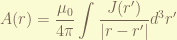
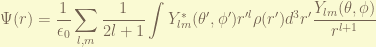
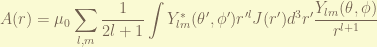
Substitute this homogeneous harmonics into the Laplace equation, the $\nabla_r^2$ will produce a coefficient related to the order, and the radial part can be extracted.

$0 = f(r) ( \nabla_\Omega^2 - g(n) ) \Theta(\Omega)$

we have an eigenvalue problem for the angular part

$\nabla_\Omega^2 \Theta = g(n) \Theta$

The eigen function for 2-D Laplacian is the Fourier Series, and that for 3-D is the Spherical Harmonics. In this sense, Fourier Series is a “polar harmonics”.

In 3-D, the angular part of the Lapacian is proportional to the angular momentum operator, $-\hbar^2 \nabla_\Omega^2 = L^2$ , where $\hbar$ is the reduced Planck constant, which has the dimension of angular momentum.

$L^2 Y_{lm}(\theta, \phi) = l(l+1) \hbar^2 Y_{lm}(\theta, \phi)$

Here, from the previous discussion, before we solve the equation, we know that the harmonic has maximum order of $l$ . The $m$ is the degeneracy for same eigenvalue $l(l+1)$

As we mentioned before, the harmonics should be rotational invariant, such that any direction should be equal. However, when we look at the Spherical Harmonics, the poles are clearly two special points and the rotation around the “z-axis” has limited rotational symmetry with degree $l$ . How come?

According to the article, the solution is not necessarily to be separated into $\theta, \phi$ , such that

$\displaystyle Y_{lm}(\theta,\phi) = \sqrt{\frac{2l+1}{4\pi} \frac{(l-m)!}{(l+m)!}}P_{lm}(\cos\theta) e^{im\phi}$

I quote the original,

“It is not immediately obvious that we can separate variables and assume exponential functions in the φ direction. We are able to do this essentially because the lines of fixed θ are circles. We could also simply assume this form and show the construction succeeds. This organization is not forced, but separating the variables is so useful that there are no competitive options. A disadvantage of this organization is that it makes the poles into special points.”

The limited rotational symmetry with degree of $l$ is due to the limited “band-width” that restricted by the order of the homogeneous function. The relation between the band width and the order of the harmonics can be understood that the number of “sector” or “node” on the circle/sphere is proportional to the order, thus, the “resolution” is also limited by the order and thus the “band-width”.

Since the Platonic solid is coordinate-free that they are the most symmetry. In the next post, I will show the relation between Spherical Harmonics and Platonic solid. This is related to the section 3.2 in the article,

“One would like to have an uniform discretization for the sphere, with all portions equally represented. From such an uniform discretization we could construct a platonic solid. It is known, however, that there are only a few platonic solids, and the largest number of faces is 20 (icosohedron) and largest number of vertices is 20 (dodecahedron). If we want to discretize the sphere with many points, we cannot do it uniformly. Instead we set the goal of using the fewest points to resolve the Spherical Harmonics up to some degree. Since the Spherical Harmonics themselves are “fair” and “uniform”, this gives a good representation for functions on the sphere. “

As the Fourier Series and Spherical Harmonic are closely related, they should share many properties. For instant, they are orthonormal and form a basis. This leads to the Discrete Fourier Transform and also the “Spherical Transform”,

$\displaystyle f(\Omega) = \sum_{\alpha} a_\alpha \Theta_\alpha(\Omega)$

where $\alpha$ is the id of the basis. One can use the Parseval theorem,

$\displaystyle \int |f(\Omega)|^2 d\Omega = \sum_{\alpha} a_\alpha^2$

Also, the convolution using discrete Fourier transform can also be applied on the spherical harmonics.

Notice that, the Discrete Fourier Transform can “translate” to Continuous Fourier Transform. However, the order of the spherical harmonics is always discrete.

Integration formulas of spherical harmonic

August 10, 2017

GoLuckyRyan Basic 3-j Symbol, spherical harmonic Leave a comment

There are several important and useful formulas for the integration of spherical harmonic. We simplify the notation,

$\displaystyle \int_0^{\pi} \sin(\theta)d\theta\int_0^{2\pi}d\phi = \int d\Omega$

The first one is the average of spherical harmonic.

$\displaystyle \int Y_{lm} d\Omega = \sqrt{4\pi} \delta_{l0}\delta_{m0}$

The 2nd one is the orthonormal condition.

$\displaystyle \int Y^{*}_{l'm'}Y_{lm} d\Omega = \delta_{l'l}\delta_{m'm}$

The 3rd one is triplet integral, we use the product of spherical harmonic,

$\displaystyle \int Y_{l_1m_1}Y_{l_2m_2} Y^*_{l_3m_3} d\Omega \\ = \int \sum_{lm} \sqrt{\frac{(2l_1+1)(2l_2+1)}{4\pi(2l+1)}} C_{l_10l_20}^{l0} C_{l_1m_1l_2m_2}^{lm} Y_{lm} Y^*_{l_3m_3} d\Omega \\= \sqrt{\frac{(2l_1+1)(2l_2+1)}{4\pi(2l_3+1)}} C_{l_10l_20}^{l_30} C_{l_1m_1l_2m_2}^{l_3m_3}$

The 4th one is another triple integral,

$\displaystyle \int Y_{l_1m_1}Y_{l_2m_2} Y_{l_3m_3} d\Omega \\ = \int \sum_{lm} \sqrt{\frac{(2l_1+1)(2l_2+1)}{4\pi(2l+1)}} C_{l_10l_20}^{l0} C_{l_1m_1l_2m_2}^{lm} Y_{lm} Y_{l_3m_3} d\Omega \\ = \int \sum_{lmLM} \sqrt{\frac{(2l_1+1)(2l_2+1)}{4\pi(2l+1)}} C_{l_10l_20}^{l0} C_{l_1m_1l_2m_2}^{lm} \\ \sqrt{\frac{(2l+1)(2l_3+1)}{4\pi(2L+1)}} C_{l0l_30}^{L0} C_{lml_3m_3}^{LM}Y_{LM}d\Omega$

$\displaystyle = \sum_{lm} \sqrt{\frac{(2l_1+1)(2l_2+1)(2l_3+1)}{4\pi}} C_{l_10l_20}^{l0} C_{l_1m_1l_2m_2}^{lm} C_{l0l_30}^{00} C_{lml_3m_3}^{00}$

Notice that

$C_{lmLM}^{00} = (-1)^{L+M} \sqrt{\frac{1}{2L+1}} \delta_{Ll}\delta_{-m,M}$

$\displaystyle \int Y_{l_1m_1}Y_{l_2m_2} Y_{l_3m_3} d\Omega = \sqrt{\frac{(2l_1+1)(2l_2+1)}{4\pi (2l_3+1)}} C_{l_10l_20}^{l_30} C_{l_1m_1l_2m_2}^{l_3,-m_3} (-1)^{m_3}$

using Wigner 3-j symbol,

$C_{l_1m_1l_2m_2}^{l_3m_3} = (-1)^{l_1-l_2+m_3} \sqrt{2l_3+1} \begin{pmatrix} l_1 & l_2 & l_3 \\ m_1 & m_2 & -m_3 \end{pmatrix}$

$\displaystyle \int Y_{l_1m_1}Y_{l_2m_2} Y_{l_3m_3} d\Omega \\= \sqrt{\frac{(2l_1+1)(2l_2+1)(2l_3+1)}{4\pi}} \begin{pmatrix} l_1 & l_2 & l_3 \\ 0 & 0 & 0 \end{pmatrix} \begin{pmatrix} l_1 & l_2 & l_3 \\ m_1 & m_2 & m_3 \end{pmatrix}$

For other integral, we can use

$Y^*_{lm}(\theta, \phi) = (-1)^{m}Y_{l(-m)}(\theta,\phi) = Y_{lm}(\theta, -\phi)$

Product of Spherical Harmonics

August 8, 2017

GoLuckyRyan Basic Clebsch-Gordon, rotation, spherical harmonic, Wigner-D Leave a comment

One mistake I made is that

$\displaystyle Y_{LM} = \sum_{m_1 m_2} C_{j_1m_1j_2 m_2}^{LM} Y_{j_1m_1} Y_{j_2m_2}$

because

$\displaystyle |j_1j_2JM\rangle = \sum_{m_1m_2} C_{j_1m_1j_2 m_2}^{LM} |j_1m_1\rangle |j_2m_2\rangle$

but this application is wrong.

The main reason is that, the $|j_1j_2JM\rangle$ is “living” in a tensor product space, while $|jm \rangle$ is living in ordinary space.

We can also see that, the norm of left side is 1, but the norm of the right side is not.

Using the Clebsch-Gordon series, we can deduce the product of spherical harmonics.

First, we need to know the relationship between the Wigner D-matrix and spherical harmonics. Using the equation

$\displaystyle Y_{lm}(R(\hat{r})) = \sum_{m'} Y_{lm'}(\hat{r}) D_{m'm}^{l}(R)$

We can set $\hat{r} = \hat{z}$ and $R(\hat{x}) = \hat{r}$

$Y_{lm}(\hat{z}) = Y_{lm}(0, 0) = \sqrt{\frac{2l+1}{4\pi}} \delta_{m0}$

Thus,

$\displaystyle Y_{lm}(\hat{r}) = \sqrt{\frac{2l+1}{4\pi}} D_{0m}^{l}(R)$

$\Rightarrow D_{0m}^{l} = \sqrt{\frac{4\pi}{2l+1}} Y_{lm}(\hat{r})$

Now, recall the Clebsch-Gordon series,

$\displaystyle D_{m_1N_1}^{j_1} D_{m_2 N_2}^{j_2} = \sum_{jm} \sum_{M} C_{j_1m_1j_2m_2}^{jM} C_{j_1N_1j_2N_2}^{jm} D_{Mm}^{j}$

set $m_1 = m_2 = M= 0$

$\displaystyle D_{0N_1}^{j_1} D_{0 N_2}^{j_2} = \sum_{jm} C_{j_10j_20}^{j0} C_{j_1N_1j_2N_2}^{jm} D_{0m}^{j}$

rename some labels

$\displaystyle Y_{l_1m_1} Y_{l_2m_2} = \sum_{lm} \sqrt{\frac{(2l_1+1)(2l_2+1)}{4\pi(2l+1)}} C_{l_10l_20}^{l0} C_{l_1m_1l_2m_2}^{lm} Y_{lm}$

We can multiply both side by $C_{l_1m_1l_2m_2}^{LM}$ and sum over $m_1, m_2$ , using

$\displaystyle \sum_{m_1m_2} C_{l_1m_1l_2m_2}^{lm}C_{l_1m_1l_2m_2}^{LM} = \delta_{mM} \delta_{lL}$

$\displaystyle \sum_{m_1m_2} C_{l_1m_1l_2m_2}^{LM} Y_{l_1m_1} Y_{l_2m_2} = \sqrt{\frac{(2l_1+1)(2l_2+1)}{4\pi(2L+1)}} C_{l_10l_20}^{l0} Y_{LM}$

From the Clebsch-Gordan coefficient, all m-values are zero, that mean the projections on the z-axis are zero for all angular momentum, thus, $l_1 + l_2 = L + even$ or $|l_1 \pm l_2 |=L$ or $l_1 + l_2 + L = even$ .

In Mathematica,

FunctionExpand[Sum[ClebschGordan[{l1, m1}, {l2, m2}, {L, M} ] SphericalHarmonicY[l1, m1, \[Theta], \[Phi]] SphericalHarmonicY[l2, m2, \[Theta], \[Phi]], {m1, -l1, l1, 1 }, {m2, -l2, l2, 1}]]
FunctionExpand[ Sqrt[((2 l1 + 1) (2 l2 + 1))/(4 \[Pi] (2 L + 1))] ClebschGordan[{l1, 0}, {l2, 0}, {L, 0}] SphericalHarmonicY[ L, M, \[Theta], \[Phi]]]

Rotation of Spherical Harmonic

June 22, 2017

GoLuckyRyan Basic Eigen System, rotation, spherical harmonic, Wigner-D Leave a comment

Rotation of a vector is easy and straight forward, just apply a rotation matrix on the vector. But rotating a function may be tricky, we need to transform the coordinate one by one.

$r \rightarrow r' = R\cdot r$

$\displaystyle f(r) \rightarrow f(r')$

When rotating spherical harmonic, the thing becomes get. We can treat the spherical harmonic as a eigen state of angular momentum operator. The problem will becomes easy.

Recall that, the rotation operator for a eigen-state is

$\displaystyle R(\alpha, \theta, \phi) = e^{-i\alpha J_z} e^{-i\theta J_y} e^{-i \phi J_z}$ ,

The matrix element is the Wigner D-matrix,

$D^j_{m'm} = \left<jm'|R|jm\right>$

The spherical harmonic is $Y_{lm}(\Omega)$

Thus, the rotation of spherical harmonic is

$\displaystyle R(Y_{lm}) = \sum_{m=-j}^{j} Y_{lm'} D^j_{m'm}$

$Y'_{l} = Y_{l} \cdot D_{l}(R)$

The above picture is $Y_{20}$ rotated by $\theta = 45 \deg$ .

We can see, the spherical harmonic formed a close set under Wigner D-matrix, that combination of them are themselves.

The derivation is follow. Notice that

$Y_{lm} = \langle \hat{r} | lm\rangle$

$\langle \hat{r}| U(R) = \langle R(\hat{r}) |$

Thus,

$Y_{lm}(R(\hat{r})) = \langle R(\hat{r}) |lm\rangle = \langle \hat{r} |U(R) |lm \rangle$

We can use the identity

$\sum_{m'} |lm'\rangle \langle lm' | = 1$

$\displaystyle Y_{lm}(R(\hat{r})) = \sum_{m'} \langle \hat{r} | lm' \rangle \langle lm' |U(R) |lm \rangle$

Than

$\displaystyle Y_{lm}(R(\hat{r})) = \sum_{m'} Y_{lm'}(\hat{r}) D_{m'm}^{l}(R)$

$Y'_{l} = Y_{l} \cdot D_{l}(R)$

It is easy to show that

$(D_{m'm}^{l}(R))^{\dagger} = D_{mm'}^{l*}(R) = D_{m'm}^l(R^{-1})$

$D_{l}^{\dagger} = D_{l}^{T*}$

Note that

$D_{l} ^{\dagger} \cdot D_{l} = 1 = D_{l} \cdot D_{l} ^{\dagger}$

spin 1 and vector

May 11, 2011

GoLuckyRyan Basic, Spherical Stuffs, theory spherical harmonic Leave a comment

the angular momentum operator L has follow properties:

$L^2 \left| l, m \right> = l(l+1) \hbar \left|l,m\right>$

$L_z \left |l,m \right> = m \hbar \left|l, m \right>$

for a spin 1 operator, we know that it is 3 dimensional. thus:

$S^2\left|m\right>=2\left|m\right>$

$S_z\left |m\right>=m\left|m\right>$

Thus, we have:

$L^2(l=1) = \frac{\hbar}{2} S^2$

where the size of L is narrowed to l =1 .

with a position bra act from the left, the L becomes:

$L^2 Y_l^m = l(l+1) \hbar Y_l^m$

$L_z Y_l^m = m \hbar Y_l^m$

$Y_l^m = \sqrt{\frac{3}{4 \pi}} \left< \hat{r} | l,m \right>$

on the counter part of spin 1 operator, the ket can be replaced by a real vector. and for any vector v, we can expand it by the 3 eigenvectors:

$\vec{v} = \left| v \right> = \sum \left|m \right> \left< m| v \right> = \sum v_m \left|m\right>$

thus, we suitable constant, a unit vector can be written in:

$\hat{r} =\sqrt{\frac{4\pi}{3}}\sum\left|m\right>Y_1^{m *}$

this is how the spherical harmonic enter the vector and then, later in matrix, and become operator.

Electromagnetic multi-pole moment

March 7, 2011

GoLuckyRyan Basic, Porperties, theory charge, dipole, Electromagnetic, moment, monopole, multipole, parity, quadrupole, spherical harmonic, vector potential 5 Comments

Electromagnetic multipole comes from the charge and current distribution of the nucleons.

Magnetic multipole in the nucleus has 2 origins, one is the spin of the nucleons, and another is the relative orbital motion of the nucleons. the magnetic charge or monopoles either do not exist or are very small. the next one is the magnetic dipole, which causes by the current loop of protons.

Electric multipole is solely by the proton charge.

From electromagnetism, we knew that the multipole has different radial properties, from the potential of the fields:

$\displaystyle \Psi(r) = \frac{1}{4\pi\epsilon_0} \int\frac{\rho(r')}{|r-r'|}d^3r'$

$\displaystyle A(r) = \frac{\mu_0}{4\pi}\int\frac{J(r')}{|r-r'|}d^3r'$

and expand them into spherical harmonic by using:

$\displaystyle \frac{1}{|r-r'|} = 4\pi\sum_{l=0}^{\infty}\sum_{m=-l}^{m=l} \frac{1}{2l+1}\frac{r_{<}^l}{r_>^{l+1}} Y_{lm}^*(\theta',\phi')Y_{lm}(\theta,\phi)$

we have

$\displaystyle \Psi(r) = \frac{1}{\epsilon_0} \sum_{l,m}\frac{1}{2l+1}\int Y_{lm}^*(\theta',\phi') r'^l\rho(r')d^3r' \frac{Y_{lm}(\theta,\phi)}{r^{l+1}}$

$\displaystyle A(r)=\mu_0 \sum_{l,m}\frac{1}{2l+1}\int Y_{lm}^*(\theta',\phi') r'^l J(r') d^3r' \frac{Y_{lm}(\theta,\phi)}{r^{l+1}}$

we can see the integral gives us the required multipole moment. the magnetic and electric are just different by the charge density and the current density. we summarize in this way :

$\displaystyle q_{lm} = \int Y^*_{lm}(\theta',\phi') r'^l \O(r') d^3 r'$

where O can be either charge or current density. The l determines the order of multipole. and the potential will be simplified :

$\displaystyle M(r)=\sum_{l,m}\frac{1}{2l+1} q_{lm} \frac{Y_{lm}(\theta,\phi)}{r^{l+1}}$

where M can be either electric or magnetic potential, and I dropped the constant. since the field is given by 1st derivative, thus we have:

monopole has $1/r^2$ dependence
dipole has $1/r^3$
quadrapole has $1/r^4$
and so on

The above radial dependences are the same for electric or magnetic. for an easy name of the multipole, we use L-pole, in which L can be 0 for the monopole, 1 for the dipole, 2 for the quadrupole, etc.. and we use E0 for the electric monopole, M0 for the magnetic monopole.

Since the nucleus must preserve parity, the parity for the electric and magnetic moment is diffident. the difference comes from the charge density and current density have different parity. The parity for charge density is even, but the current density is odd. $1/r^2$ has even parity, $1/r^3$ has odd parity. therefore

electric L-pole — $(-1)^{L}$
magnetic L-pole — $(-1)^{L+1}$

for easy comparison:

E0, E2, E4… and M1,M3, M5 … are even
E1,E3,E5…. and M0, M2, M4…. are odd

The expectation value for L-pole, we have to calculate :

$\displaystyle \int \psi^* Q_{lm} \psi dx$

where $Q_{lm}$ is a multipole operator ( which is NOT $q_{lm}$ ), and its parity is follow the same rule. the parity of the wave function will be canceled out due to the square of itself. thus, only even parity are non-Zero. those are:

E0, E2, E4…
M1,M3, M5 …

that makes sense, think about a proton orbits in a circular loop, which is the case for E1, in time-average, the dipole momentum should be zero.

Nuclear Physics 101

Coulomb Energy for two protons system

Evaluation of mutual interaction

Review on rotation

Spherical Harmonics and Platonic Solids

Spherical Harmonics and Fourier Series

Integration formulas of spherical harmonic

Product of Spherical Harmonics

Rotation of Spherical Harmonic

spin 1 and vector

Electromagnetic multi-pole moment

Recent Posts

Calendar

Archives

Keywords

# of Visitors

Login