The Gamma Transition is on this post, but it seems that the equation connecting transition rate and reduced transition rate missed a factor
The relations between mean lifetime , half-life , (partial) decay width , and transition rate are:
The gamma transition rate in s-1 is related to the electric reduced transition rate in e2fm2L is:
Here is a table for the first few coefficients
Multiple
Decay rate (1/s), in MeV
E1
B(E1) [e2fm2]
E2
B(E2) [e2fm4]
E3
B(E3) [e2fm6]
E4
B(E4) [e2fm8]
E5
B(E5) [e2fm10]
The reduced decay rate and reduced excite rate is related by:
For example, in 10C, the first 2+ (3.354 MeV) to 0+ (g.s.) has mean lifetime of 219 fs (E. A. McCutchan et al., PRC 86, 014312 (2012)), the transition rate is then s-1, and the decay width is 3.01 meV. As this is 100% E2 decay, using the above formula, the B(E2) is 8.781 e2fm4. And the excite B(E2; 0+ -> 2+) is 5 times larger.
How does a Poisson process generate the exponential decay?
The exponential decay is derived by
which means the rate of the loss of the number of nuclei is proportional to the number of nuclei. and is the half-life.
This is a phenomenological and macroscopic equation that tells us nothing about an individual decay.
Can we have a microscopic derivation that, assumes the decay of an individual nucleus following a random distribution?
From this post, we derived the distribution for the differences in a list of sequential random numbers. The key idea is the probability of having a decay at exactly time to , denote as , is
where is the probability of having decay within (time) length , which is a Poisson distribution.
Now, the total probability of all possible decay within time , assume not more than 1 decay can happen in ,
Thus, the number of nucleus not decay or survived within time is
Suppose the radioisotope has half-life of and initial number of , the number of isotopes at give time is
The number of decay at a given time, measured with a time period is
The rate of number of decay at a given time is
or
This, the rate of number of decay is always proportional to the number of radioactive isotopes, therefore, by measuring the radioactivity, the number of radioactive isotopes can be deduced.
For example, suppose we have a sample of tritium with half live of sec. When we measure the sample, we got 100 beta decay in 1 min, that means, the radioactivity is 1.67 decay per second. Therefore the number of isotopes is tritium. Notice that, this number is the number of isotopes at the end of measurement.
For very short half-life, say, few mili-sec, if we collect the number of decay in a few seconds, the number of isotopes changed a lot and the simple ratio is no longer accurate.
I revisit the NMR theory and technical stuff. Doing a 90 degrees flip and measure the Free Induction Decay (FID) signal. The NMR theory is simple, under a magnetic field, the proton spin is precessingat the Larmor frequency, but the spin aligns with the field (alone the z-axis) and the change of the magnetic field on the x-y plane is very weak. To increase the change of the magnetic field, we can flip the spin 90 degrees, make it precesses on the x-y plane and maximize the change of the magnetic field. With the change of the magnetic field induct electric field and voltage on a coil (on the x-axis for example), an signal can be detected at the Larmor frequency. Since the spin will graduate align itself back to the z-axis and so the signal will decay. The technique to flip the spin is called Nuclear Magnetic Resonance. I made a very clumsy note on that many years ago in this pdf.
In order to flip the spin, we need to apply a rotating field with frequency , in the rotating frame created by the rotating field, an inducted field is created alone the negative z-axis as the world is rotating around (in an opposite direction), and also, a constant field points along the rotating x-axis. When the induced field in the rotating frame can cancel the external magnetic field, the over all effective magnetic field would be the one along the rotating x-axis. Since nuclear spin was on the z-axis, and since switch on of the rotating field, it feels a net magnetic field along the rotating x-axis and start to precess around it. If the rotating field switch off at the time that the spin precesses on the x-y plan, a 90 degree flip is done.
Mathematically, the Hamiltonian a spin under and external magnetic field is
where is the gyromagnetic ratio of proton, in which is the g-factor of proton and is the proton magneton. The Larmor frequency is .
with a oscillating magnetic field (which is effectively combination of a right-hand and left-hand rotating field), the Hamiltonian is
The factor represent the strength of the rotating field. The factor of 2 will comes in handy later. In order to change to the rotating frame, suppose the Lab wavefunction is , the rotating frame wavefunction is , the rotating frame Hamiltonian must satisfy
Thus,
We can drop the last time dependence terms, because it oscillate at twice of the frequency of the rotating frame, that, in average, the contribution is averaged out. And the Hamiltonian is as expected as our early discussion. an induced field along the z-axis, and constant field along the x-axis.
The strength of the oscillating field has a meaning of rotational frequency. If we apply the field so that and , this will rotate the spin 90 degree and give a maximum reading from the NRM coil. The challenge is that, the actual value of depends on the effective oscillating magnetic field strength , which depends on the power transfer from the source to the NMR coil, the impedance matching from the coil to the source, also the resonance frequency of the chamber. Some these factors are hard to measure and often, the 90 degree spin flip is achieved by trials and errors until the maximum FID is obtained.
The installation in Ubuntu 22.04 can be found at the end of this post. The trick for the installation is enabling visualization. The one I pick is the Qt OpenGL, and it requires to have Qt installation.
To install Qt, I download the Qt installer from the Qt website. In the installer, I pick the manual components to install. The components are
The nature of the spectroscopic factor is discussed here (from the point of view of mean-field) and here (from an experimental point of view). Here are some updates and additional discussions on the topic.
Up to now, I still believe that the quenching of the SF simply reflects the mismatch between experiment and theory, due to experimental conditions that limited configurations can be observed (so that the sum of SF is less than 1), and also the reaction theory does not take into account the correlation (so that the SF of each state is quenched). If both limitations are removed, there is no quenching. Although the SF is quenched, careful normalization gives us a great deal about the nuclear structure.
Is the spectroscopic factor or the cross-section quenched?
It seems that since the spectroscopic factor and the cross-section are closely related by
so, the question is meaningless, because when SF is quenched from unity, the cross-section is also quenched from the therotical cross-section. However, since cross-section is an observable while SF is not, people consider that it is more proper to say quenching of cross-section.
However, I think SF is an observable because there should be a natural basis and fixed interaction. when the basis is fixed, and the 1st order of the nuclear interaction is well-known, the SF is well-defined, just like the coefficient of fractional percentage. Another argument is that there are many articles on extracting the spectroscopic factors, and although the uncertainty can be as large as 50% due to various experimental conditions and analysis methods, the community has a consensus on the quenching. That is, the community reached a consensus on the basis and range of interaction. I think that means, we are reaching the natural basis and 1st order understanding of the interaction.
The situation is like if we have the theoretical framework but lack some fundamental parameters fixed. The theory can produce all kinds of phenomena. Say, neutrino mass, without that, we don’t know the neutrino mass hierarchy. But we cannot say the neutrino mass hierarchy should fall in either the normal or inverted hierarchy and therefore neutrino mass hierarchy is not well-defined. My point is once the nuclear interaction and the basis are fixed, the SF is uniquely determined. So, some people would say, SF is an quasi-observable and that it is not an observable yet, but it will. May be, we should call SF is an extractable/deductible, which is a extractable/deductible quantity with some will-be-fixed parameter sets.
The last comment is that, if SF is not an observable, and is a pure arbitrary construct, all the works on it become meaningless. But, I believe SF is not aether, it reveals the structure and nucleon configuration of a nucleus. Also, the effective single-particle energy (ESPE) is an SF weighted energy of an orbital. If SF is arbitrarily constructed and can be anything, so the ESPE. but the ESPE very much agrees with the energy levels from Woods-Saxon potential which is a 1st order approximation of the nuclear mean field. A similar thing to the asymptotic normalization coefficient (ANC), ANC is a ratio of the wavefunction to the Coulomb wave function outside the nuclear potential, and the wavefunction is not an observable, so ANC is also not. But the wavefunction is surely can be deduced/extracted from the experimental data by fixed some nuclear parameters.
So, if SF is an observable, it is meaningless to ask is SF quenched or cross-section quenched.
If, the theoretical cross-section is perfectly calculated, the SF would be unity and no quenching for either SF or cross-section, and the nucleon configuration is embedded into the coefficient of fractional percentage.
The whole discussion is on two-dimensional only. Suppose the 2 line segments are defined by points and . The 2 segments can either be parallel or non-parallel.
Non-parallel case. There are at least 2 methods to determine, straightforward thinking is to construct the equation of the 2 lines using the 2 segments
solve for the parameters . One way is using bull force to solve it. Another way is the area ratio:
The nominator is the area of the triangle . The denominator is the area of the whole area . The whole area is
The simplification uses the identity .Similarly.
The intersect condition is
In the case of parallel, there are 2 cases: with offset or without offset
In the case of offset, the “whole” area , geometrically, the cross-product as it is clockwise. Since the 2 segments are parallel, the perpendicular distances from or to line are the same. So, the area
When the 2 segments are “co-planar”, the nominator becomes zero too. To check if the two segments overlap or not, simply check x- or y-component is enough.
Haven’t posted anything for a while, was working on extracting carbon isotopes ESPS, the FSU DAQ, and SOLARIS DAQ for the NUMEN collaboration, went to Hawaii for DNP 2023, and got sick for a week…. Anyway, a friend was having trouble doing a HELIOS simulation with a non-uniform field in GEANT4, and I am curious what is the effect of a non-uniform field, so, I decided to do my own simulation. The core of the simulation is solving the Lorentz equation . This is a 2nd order coupled equation. Well, I already solved it before, so it would be not a huge work.
In this post, I already show that using RK4 method to solve the Lorentz equation. Here, I show the method using the Scipy library in Python and also NDSolve[] in Mathematica.
#Define magnetic field
def Bx(x, y, z):
  return  x/ (1 + math.exp( x**2 + y**2) )
def By(x, y, z):
  return  y/ (1 + math.exp( x**2 + y**2) )
def Bz(x, y, z):
  return -2.5 / (1 + math.exp((math.sqrt(x**2 + y**2) - 0.5)/0.05)) / (1 + math.exp((z**2 - 1**2)/0.1))

from scipy.integrate import odeint

def FieldEquations(w, t, p):
  x , y, z, vx, vy, vz = w

  f = [vx,
       vy,
       vz,
       p * ( vy * Bz(x,y,z) - vz * By(x,y,z)),
       p * ( vz * Bx(x,y,z) - vx * Bz(x,y,z)),
       p * ( vx * By(x,y,z) - vy * Bx(x,y,z))]
  return f

def SolveTrace( helios, thetaCM_deg, phiCM_deg, r0_meter, tMax_ns):
  vx0, vy0, vz0 = helios.velocity_b(thetaCM_deg, phiCM_deg)
  w0 = [r0_meter[0], r0_meter[1], r0_meter[2], vx0, vy0, vz0]

  # ODE solver parameters
  abserr = 1.0e-8
  relerr = 1.0e-6
  stoptime = tMax_ns
  numpoints = 500

  # Create the time samples for the output of the ODE solver.
  t = [stoptime * float(i) / (numpoints - 1) for i in range(numpoints)]

  wsol = odeint(FieldEquations, w0, t, args=(helios.QMb,), atol=abserr, rtol=relerr)

  return [t, wsol]
The code is very simple, we first define the magnetic field components, next, in the FieldEquation, the w is the coordinate vector, and f is the corresponding equation for the coordinate vector, for the x-component, which is
Similar for the y- and z-components. The variable p is the charge-to-mass ratio. The SolveTrace will use the helios class, which is not shown here, but it basically gives the velocity vector for the initial velocity. The output is the list of the time and the wsol. the wsol is an array of array of x, y, z, vx, vy, and vz.
The code defines the field components first, the G2x is the . After that, use the NDSolve to solve for .
A small note on the unit. We are going to solve it in units of meters and nano-seconds. So, the initial position and velocity are in meter and meter/nano-sec respectively. and the charge-to-mass ratio is in SI unit, so, using Coulomb over kg. The charge-to-mass ratio also needs to be multiplied by because the left-hand side is 2nd derivative of time in nano-sec, while the right-hand side needs to be multiplied by to give the correct scale. (think about the original Lorentz equation is in mater and sec)
Now, we are in a position to solve the locus of the charged particle for any field. In particular, I like to find out the effect of a radial component.
I set the radial field to be , where is the strength of the radial component. The radial field is strong at small and decay with .
For the reaction, I pick 15N(d,p) at 10 MeV/u. At , The velocity vector is [meter/ns]. The locus when is
Interestingly, the particle experiences a positive z-acceleration. Imagine the particle only moves in the x-y plane, with a radial component of the field, the particle experiences a positive z-force.
Another effect is the distortion of the x-y projection. Without the radial field, the x-y projection should be a perfect circle. Since the radial field gives a +z-force, and the z-field gives a radially inward force. These two forces combined will twist the path.
Here is the locus for
as expected, a stronger radial field, the stronger positive z-force, and the particle change the moving direction more quickly. Also, the x-y project is more distorted.
A spectrograph relates the measured momentum to the excitation energy of the heavy recoil, assuming that the light recoil does not excite. In a two-body transfer reaction, there are 3 degrees of freedom, 2 from the scattering angle, and 1 from the excited energy of the heavy recoil. In a spectrograph, the lab angle of the light recoil is fixed with a small acceptance. Thus, the momentum of the light recoil is correlated with the excitation energy of the heavy recoil.
This post is the normal kinematics of a Split-Pole spectrograph. The given condition is the angle of the Split-Pole, the mass of all 4 particles, and the excitation energy of the heavy recoil. In the classical limit, the conservations of KE and momentum are,
The momentum balance is directly from the cosine law.
The job is get the in term of by eliminating . Obviously,
Rearrange,
Thus, the is
When , the sqrt root is always valid, and always has 2 solutions.
We are interested in the forward center of mass angle, so we take the higher value of .
For a magnetic field , the radius is
If the mass is in MeV/c^2, we have
We can also do it in relativistic way. The conservation of energy and momentum give
The momentum balance is done by cosine law. Solve for ,
With the momentum of the light recoil particle in MeV/c, the cyclotron radius is under a magnetic field strength in T is
An interesting case is when , i.e. like a head-on collision. In that case, the mass of b is, by solving ,
I am not sure what does it means…
The Split-pole spectrograph measures the cyclotron radius for various states of particle b, assuming particle a does not excited. i.e. . Since is a constant, if we can find the formula to convert back to , what would be very nice.
Solve for using the relativistic equation of , or consider the energy and momentum balance
square the , the mass of b is
using to replace , we have
Here is a plot for 12C(d,p) at 10 MeV/u at 10 degree. The equation is


 in MeV
 B(E1) [e2fm2]
 B(E2) [e2fm4]
 B(E3) [e2fm6]
 B(E4) [e2fm8]
 B(E5) [e2fm10]


 is the half-life.
 to
to  , denote as
  , is
, is
 is the probability of having
  decay within (time) length

 ,
,
 is
is
 , the number of isotopes at give time is
 is
is 


 sec. When we measure the sample, we got 100 beta decay in 1 min, that means, the radioactivity is 1.67 decay per second. Therefore the number of isotopes is
  tritium. Notice that, this number is the number of isotopes at the end of measurement.
 is no longer accurate.

 , in the rotating frame created by the rotating field, an inducted field is created alone the negative z-axis as the world is rotating around (in an opposite direction), and also, a constant field points along the rotating x-axis. When the induced field in the rotating frame can cancel the external magnetic field, the over all effective magnetic field would be the one along the rotating x-axis. Since nuclear spin was on the z-axis, and since switch on of the rotating field, it feels a net magnetic field along the rotating x-axis and start to precess around it. If the rotating field switch off at the time that the spin precesses on the x-y plan, a 90 degree flip is done.
 is the gyromagnetic ratio of proton, in which
  is the g-factor of proton and
  is the proton magneton. The Larmor frequency is
  .
.
 , the rotating frame wavefunction is
  , the rotating frame Hamiltonian must satisfy
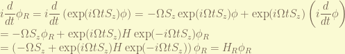

 along the z-axis, and constant field along the x-axis.
  and
and  , this will rotate the spin 90 degree and give a maximum reading from the NRM coil. The challenge is that, the actual value of
  depends on the effective oscillating magnetic field strength
  , which depends on the power transfer from the source to the NMR coil, the impedance matching from the coil to the source, also the resonance frequency of the chamber. Some these factors are hard to measure and often, the 90 degree spin flip is achieved by trials and errors until the maximum FID is obtained.

 and
and  . The 2 segments can either be parallel or non-parallel.
 . One way is using bull force to solve it. Another way is the area ratio:

 . The denominator is the area of the whole area
  . The whole area is
 .Similarly.


 , geometrically, the cross-product
  as it is clockwise. Since the 2 segments are parallel, the perpendicular distances from
  or
or  to line
  are the same. So, the area


 . This is a 2nd order coupled equation. Well, I already solved it before, so it would be not a huge work.
 . After that, use the NDSolve to solve for
  .
.  because the left-hand side is 2nd derivative of time in nano-sec, while the right-hand side needs to be multiplied by
  , where
  and decay with
 , The velocity vector is
  [meter/ns]. The locus when
  is
is 


 in term of
  by eliminating
  . Obviously,


 , the sqrt root is always valid, and
  , the radius is


 ,
,

![\displaystyle \rho [\textrm{m}] = \frac{k_a [\textrm{MeV/c}] }{ c q B [\textrm{T}]}, ~~ c = 299.792458](https://s0.wp.com/latex.php?latex=%5Cdisplaystyle+%5Crho+%5B%5Ctextrm%7Bm%7D%5D+%3D+%5Cfrac%7Bk_a+%5B%5Ctextrm%7BMeV%2Fc%7D%5D+%7D%7B+c+q+B+%5B%5Ctextrm%7BT%7D%5D%7D%2C++%7E%7E+c+%3D+299.792458+&bg=fafad3&fg=6f5e4e&s=0&c=20201002)
 , i.e. like a head-on collision. In that case, the mass of b is, by solving
  ,
, 
 . Since
  is a constant, if we can find the formula to convert
  back to
  , what would be very nice.
  using the relativistic equation of
 , the mass of b is

 to replace
  , we have


 is in SI unit,


 . We have:


 in the 2nd equation because we have to subtract
  at the end.

 from either case is


 .
. 
