I found that most of the book only talk part of it or present it separately. Now, I am going to treat it at 1 place. And I will give numerical value as well. the following context is on SI unit.
a very central idea when writing down the state quantum number is, is it a good quantum number? a good quantum number means that its operator commute with the Hamiltonian. and the eigenstate states are stationary or the invariant of motion. the prove on the commutation relation will be on some post later. i don’t want to make this post too long, and with hyperlink, it is more reader-friendly. since somebody may like to go deeper, down to the cornerstone. but some may like to have a general review.
the Hamiltonian of a isolated hydrogen atom is given by fews terms, deceasing by their strength.

the Hamiltonian can be separated into 3 classes.
__________________________________________________________
Bohr model
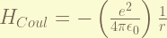
is the Coulomb potential, which dominate the energy. recalled that the ground state energy is -13.6 eV. and it is equal to half of the Coulomb potential energy, thus, the energy is about 27.2 eV, for ground state.
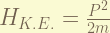
is the non-relativistic kinetic energy, it magnitude is half of the Coulomb potential, so, it is 13.6 eV, for ground state.
comment on this level
this 2 terms are consider in the Bohr model, the quantum number, which describe the state of the quantum state, are
 = principle number. the energy level.
 = orbital angular momentum. this give the degeneracy of each energy level.
 = magnetic angular momentum.
it is reasonable to have 3 parameters to describe a state of electron. each parameter gives 1 degree of freedom. and a electron in space have 3. thus, change of basis will not change the degree of freedom. The mathematic for these are good quantum number and the eigenstate  is invariant of motion, will be explain in later post. But it is very easy to understand why the angular momentum is invariant, since the electron is under a central force, no torque on it. and the magnetic angular momentum is an invariant can also been understood by there is no magnetic field.
the principle quantum number  is an invariance. because it is the eigenstate state of the principle Hamiltonian( the total Hamiltonian )!
the center of mass also introduced to make more correct result prediction on energy level. but it is just minor and not much new physics in it.
Fine structure
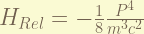
is the 1st order correction of the relativistic kinetic energy. from  , the zero-order term is the non-relativistic kinetic energy. the 1st order therm is the in here. the magnitude is about
  . ( the order has to be recalculate, i think i am wrong. )
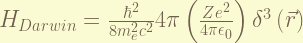
is the Darwin-term. this term is result from the zitterbewegung, or rapid quantum oscillations of the electron. it is interesting that this term only affect the S-orbit. To understand it require Quantization of electromagnetic field, which i don’t know. the magnitude of this term is about 
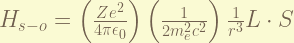
is the Spin-Orbital coupling term. this express the magnetic field generated by the proton while it orbiting around the electron when taking electron’s moving frame. the magnitude of this term is about 
comment on this level
this fine structure was explained by P.M.Dirac on the Dirac equation. The Dirac equation found that the spin was automatically come out due to special relativistic effect. the quantum number in this stage are
= principle quantum number does not affected.
= orbital angular momentum.
= magnetic total angular momentum.
 = spin angular momentum. since s is always half for electron, we usually omit it. since it does not give any degree of freedom.
 = magnetic total angular momentum.
at this stage, the state can be stated by  , which shown all the degree of freedom an electron can possible have.
However,  is no longer a good quantum number. it does not commute with the Hamiltonian. so, does not be the eigenstate anymore. the total angular momentum was introduced
  . and
. and  and
and  commute with the Hamiltonian. therefore,
 = total angular momentum.
 = magnetic total angular momentum.
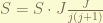
an eigenstate can be stated as  . in spectroscopy, we denote it as
  , where
  is the spectroscopy notation for .
there are 5 degrees of freedom, but in fact, s always half, so, there are only 4 real degree of freedom, which is imposed by the spin ( can up and down). the reason for stating the s in the eigenstate is for general discussion. when there are 2 electrons, s can be different and this is 1 degree of freedom.
Hyperfine Structure
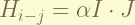
is the nuclear spin- electron total angular momentum coupling. the coefficient of this term, i don’t know. Sorry. the nuclear has spin, and this spin react with the magnetic field generate by the electron. the magnitude is 

is the lamb shift, which also only affect the S-orbit.the magnitude is 
comment on this level
the hyperfine structure always makes alot questions in my mind. the immediate question is why not separate the orbital angular momentum and the electron spin angular momentum? why they first combined together, then interact with the nuclear spin?
may be i open another post to talk about.
The quantum number are:
= principle quantum number
= orbital angular momentum
= electron spin angular momentum.
= spin-orbital angular momentum of electron.
 = nuclear spin. for hydrogen, it is half.
 = total angular momentum
 = total magnetic angular momentum
a quantum state is $\left| n, l, s, j,i, f , m_f \right>$. but since the s and i are always a half. so, the total degree of freedom will be 5. the nuclear spin added 1 on it.
Smaller Structure

this term is for the volume shift. the magnitude is  .
.
in diagram:


![H = -\gamma \vec{J}\cdot \vec{B} = -\gamma J_z B = -\gamma \hbar \frac{m}{2} B [J]](https://s0.wp.com/latex.php?latex=H+%3D+-%5Cgamma+%5Cvec%7BJ%7D%5Ccdot+%5Cvec%7BB%7D+%3D+-%5Cgamma+J_z+B+%3D+-%5Cgamma+%5Chbar+%5Cfrac%7Bm%7D%7B2%7D+B+%5BJ%5D&bg=fafad3&fg=6f5e4e&s=0&c=20201002)


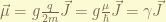
![|\vec{\mu_e}|= g_e \frac{e}{2 m_e} \frac{\hbar}{2} = \gamma_e \frac{\hbar}{2} [JT^{-1}]](https://s0.wp.com/latex.php?latex=%7C%5Cvec%7B%5Cmu_e%7D%7C%3D+g_e+%5Cfrac%7Be%7D%7B2+m_e%7D+%5Cfrac%7B%5Chbar%7D%7B2%7D+%3D+%5Cgamma_e+%5Cfrac%7B%5Chbar%7D%7B2%7D+%5BJT%5E%7B-1%7D%5D&bg=fafad3&fg=6f5e4e&s=0&c=20201002)
![\gamma_e = g_e \frac{\mu_e}{\hbar} [rad s^{-1} T^{-1}]](https://s0.wp.com/latex.php?latex=%5Cgamma_e+%3D+g_e+%5Cfrac%7B%5Cmu_e%7D%7B%5Chbar%7D+%5Brad+s%5E%7B-1%7D+T%5E%7B-1%7D%5D&bg=fafad3&fg=6f5e4e&s=0&c=20201002)


![\gamma_e = g_e \frac{\mu_e}{2\pi\hbar} [Hz T^{-1}]](https://s0.wp.com/latex.php?latex=%5Cgamma_e+%3D+g_e+%5Cfrac%7B%5Cmu_e%7D%7B2%5Cpi%5Chbar%7D+%5BHz+T%5E%7B-1%7D%5D&bg=fafad3&fg=6f5e4e&s=0&c=20201002)


 . bu measuring the amplitude with different
  .
.


 pulse, the spin go to – y axis. now, due to the incoherence of each spin, some spin are faster and some are slower. after a time
  pulse flips all the spin by 180 degree. now, the “slower” spin become ahead of the “faster” spin. After the same time interval, the “faster” spin will catch up the “slower” spin and all the spin becomes coherence at that moment again! thus, the amplitude of the signal will become large again. However, since the spins are not at same Larmor frequency, some will flip more than 180 degrees while some flip less, thus, the decay are still there.
 should be :

 , where
  is nuclear magnetron. (reference? exp?)
 and
and  , the ratio between these 2 are 1.14/3, instead of 1/3.
 . The parity transform is changing it to


 and
and  are the angle of spin . not the detector angle.


 is from the yield measurement.


 is the amplitude and
  is the Larmor frquency. for consistency and cross reference in this blog, i keep the 0 with the
  .
.


 Tesla ), a higher magnetic field strength, the higher Larmor frequency, and a stronger signal.
 , which is an internal degree of freedom to let particle “orbiting” at there.

 can be either
  .
.
 can be both half-integral and integral. the half-integral value of
  makes the spin-state have to rotate 2 cycles in order to be the same again.


 is equal to
  . the different in the c will come up at very long time measurement and it exhibit a interference pattern.
 is a complex number, it will cause a decay, and it will be reflected in the interference pattern.
![[x,S]=0 ?](https://s0.wp.com/latex.php?latex=%5Bx%2CS%5D%3D0+%3F+&bg=fafad3&fg=6f5e4e&s=0&c=20201002)
![[p,S]=0 ?](https://s0.wp.com/latex.php?latex=%5Bp%2CS%5D%3D0+%3F+&bg=fafad3&fg=6f5e4e&s=0&c=20201002)
![[p_x, S_y] \ne 0 ?](https://s0.wp.com/latex.php?latex=%5Bp_x%2C+S_y%5D+%5Cne+0+%3F+&bg=fafad3&fg=6f5e4e&s=0&c=20201002)

![[V_i, J_j] = i \hbar V_k](https://s0.wp.com/latex.php?latex=%5BV_i%2C+J_j%5D+%3D+i+%5Chbar+V_k+&bg=fafad3&fg=6f5e4e&s=0&c=20201002) run in cyclic
run in cyclic
